Model configurations for benchmarks

This page only refers to the direct problem and the description of the forward models. Model configurations of increasing complexity will be used to elaborate the benchmarks. These model configurations will include:

Small case benchmark: Lorenz-96 model

The Lorenz-96 (L96) model is defined by:

with cyclic index: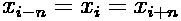

Numerics. The differential equation are solved with a fourth-order Runge-Kutta scheme with time step dt=0.05, corresponding to a geophysical time of 6h. Other specifications: n=40, F=8, and the spin-up is initialized by choosing F=8.01 at the 20th grid point (Van Leeuwen 2010).

Go to technical specifications.

Medium case benchmark: double-gyre NEMO configuration

The medium case benchmark is based on an idealized configuration of the NEMO primitive equation ocean model (as described in Cosme et al. 2010): a square and 5000-meter deep flat bottom ocean at mid latitudes (the so called square-box or SQB configuration).

Physics. In this square basin (between 25°N and 45°N), a double gyre circulation is created by a constant zonal wind forcing blowing westward in the northern and southern parts of the basin and eastward in the middle part of the basin. The domain is closed and the lateral boundaries are frictionless. The western intensification of these two gyres produces a western boundary current that feeds an eastward jet in the middle of the square basin (see figure below, showing a snapshot of the model sea surface height). This jet is unstable so that the flow is dominated by chaotic mesoscale dynamics, with largest eddies that are about 100 km wide, and to which correspond velocities of about 1 m/s and dynamic height differences of about 1 meter. All this is very similar in shape and magnitude to what is observed in the Gulf Stream (North Atlantic) or in the Kuroshio (North Pacific).

Numerics. The primitive equations are discretized on an Arakawa C grid, with a horizontal resolution of 1/4° x 1/4° cos(φ) and 11 z-coordinate levels along the vertical. The model uses a `free surface' formulation, with an additional term in the momentum equation to damp the fastest external gravity waves. Momentum advection is performed with an energy conserving numerical scheme in vector form, and tracer advection is performed with a 2nd order centered scheme. Time stepping is performed with a leap frog scheme, with a time step dt=900 s.

Go to technical specifications.

Large case benchmark: North-Atlantic 1/4° NEMO/LOBSTER configuration

The large case benchmark is based on a realistic configuration of the NEMO ocean model, for the North Atlantic Ocean, at a 1/4° resolution (Barnier et al, 2006), and including an ecosystem model component (Ourmières et al., 2009), figuring the operational MyOcean systems. This model was selected because it has been used in numerous assimilation studies before (Ourmières et al., 2009, Béal et al, 2010, Doron et al. 2011) and because it is based on the NEMO ocean model which is used by most MyOcean Monitoring and Forecasting Centres. This implementation will be used for selected simulations to assess new techniques with real data.

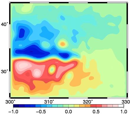
Physics. The model circulation is simulated by the OPA code using the free surface formulation. Prognostic variables are the three-dimensional velocity fields and the thermohaline variables. The model domain covers the North Atlantic basin from 20°S to 80°N and from 98°W to 23°E. The horizontal resolution is 1/4 of a degree, which is considered as eddy-permitting in the mid-latitudes where the Rossby radius of deformation is about 100 km. (see figure below, showing a snapshot of the model sea surface height). Lateral mixing of momentum and tracers is modelled with a biharmonic operator, vertical mixing is modelled by the TKE turbulence closure scheme, and convection is parameterized with enhanced diffusivity and viscosity. The forcing fluxes are calculated via bulk formulations, using the ERAnterim atmospheric forcing fields. Buffer zones are defined at the southern, northern and eastern (Mediterranean) boundaries (which are closed), with restoring to Levitus climatology.

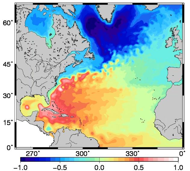
Ecosystem. The biogeochemical model used is LOBSTER (LOCEAN Biogeochemical Simulation Tool for Ecosystem and Resources). It is nitrogen-based and contains six prognostic variables: nitrate, ammonium, phytoplankton, zooplankton, detritus and semilabile dissolved organic matter. In the model, the bottom of the euphotic layer is considered to be at a constant depth of 191 m. In the euphotic layer, the biogeochemical functionalities work as described in the figure below (see Lévy et al., 2005 for more detail about the model equations). As LOBSTER features two nutrients, new production and regenerated production can be distinguished. Below the euphotic layer, the model considers very simple parameterizations of decay to nitrate, detritus sedimentation and remineralization of zooplankton mortality.

Numerics. The primitive equations are discretized on an Arakawa C grid, with a horizontal resolution of 1/4° x 1/4° cos(φ). Vertical discretization is done on 45 geopotential levels, with a grid spacing increasing from 6 m at the surface to 250 m at the bottom (with partial step to better discretize the bottom topography). The model uses a `free surface' formulation, with an additional term in the momentum equation to damp the fastest external gravity waves. Momentum advection is performed with an energy and enstrophy conserving numerical scheme in vector form, and tracer advection is performed with the TVD scheme. Time stepping is performed with a leap frog scheme, with a time step dt=2400 s. The biogeochemical model is coupled on-line to the circulation model, with a coupling frequency equal to the circulation model time step.

Go to technical specifications.